Frequency Domain Mode Profile Monitors
In today's post we are going to build a monitor capable of showing the field profile along a 2D cut of our system for any frequency within the source bandwidth after a single simulation. I find this specially useful when trying to identify the resonances of a structure. We will use a modified version of the ring resonator in the Meep tutorials to test the implementation and, by the end of the post, you will have this:
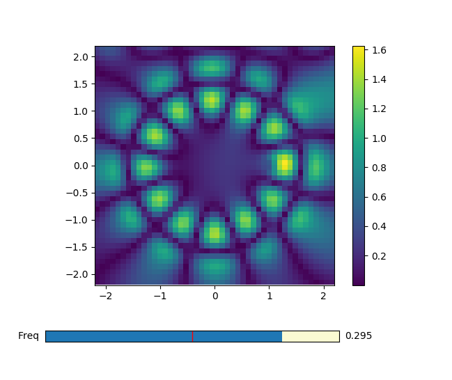
Interactive frequency monitor.
The method proposed on the Meep basic tutorials to show the fields at a specific frequency is firstly identifying the resonances of the structure using harminv, followed by a narrow bandwidth simulation. This can easily become a time consuming process if you need to look at many resonances. The monitor that we are building here will trade-off some hard disk space and a small amount of post-processing time for the convenience of being able to look at the field profile at any frequency with a single simulation.
Caution!!
Using this monitor consumes orders of magnitude more hard drive space than just outputting a snapshot of the field. File sizes can easily run over 50 MB for a not too big 2D simulation. Generalizing the method below to 3D simulations is trivial, but I've never tried it and file size for a single simulation may well go into the multiple GBs.
The size of the output file will also depend a lot on how long you acquire data. For example, if your finishing condition consists on waiting for the fields to decay by a certain amount and you are simulating a high-Q cavity, the output file will be much bigger. Of course you can control for how long you want to acquire data but still you should take it into consideration.
What you have to do is sample the field at the Nyquist
rate for the highest frequency you
are interested on. Then Fourier transform the output to disentangle the
different frequency components. Finally, you'll add additional attributes onto
the h5 file to avoid having to manually keep in sync the representation scripts
and the simulation ctl file.
Lets start with two helper functions. One generates the volume over which we
want to visualize the fields, the other creates a step function that will
output the fields into a file called monitor-name.h5 every
dt.
After running the simulation we’ll want to add some metadata to the h5 file so
that we don’t have to keep track manually of what are the dimensions of the
volume or which was the specific sampling rate. I couldn’t figure out a way of
doing this using only libctl so, instead, I created a Python script that takes
care of it. The function attr->string builds a string with the call to the
Python script in charge of adding the metadata. The Python script is then
called via the system function. Of course you can use this to append an
attribute to any h5 file.
Finally to obtain the field at each frequency run a discrete Fourier transform
on the fields. The transform is performed only along the time axis which means
that each pixel in the stored volume is treated as an independent time series.
Depending on the required frequency resolution you may need to pad the signal
with zeros. This is taken care of by the n argument of the FFT function. The
example below will plot the absolute value of whatever field was stored in the
monitor but any other function of the fields is possible.
The code available on
GitHub
includes a bash script to run the simulations and some further instructions.
You will also find a notebook to plot the LDOS of the system which should be
really helpful to hunt down the resonances. The show_freq_monitor.py
script is a small command line program that will take care of Fourier
transforming the fields in the monitor and plotting them together with a slider
to select the frequency you are interested on. Besides plotting the Fourier
transform it can also apodize the beginning of the time signal. This can be
useful if, for example, your source is dominating the output at the beginning,
which makes it hard to see anything else. The --t0 and --tau define the
center of the apodization and the characteristic time of the ramp up.
Hopefully this will provide you with a new tool in your FDTD arsenal to make your workflows more efficient.