Maxwell Rules - Monte Carlo Integration

Monte Carlo Integration

TLDR;

Monte Carlo (MC) ingegrals are a useful and cool tool that you should know about. Here are a few facts that you want to take home.

Pros:

Integral error is independent of dimensionality.
Very weak conditions are imposed on the integrand.
Easy to deal with complex boundaries of the integration domain.
Not MC specific, but still, there are great libraries that will do fast and efficiently for you.

Cons:

Error of the integral is non-deteministic.
Slow convergence $1/\sqrt(N)$. For small dimensionality quadrature method will be faster for a given accuracy.

Welcome to Monte Carlo!

Monte Carlo are a family of algorithms that are based around the use of (pseudo)randomly generated numbers in order to calculate some quantity of interest or estimate the distribution of some variable given some randomness in the input.

This post will cover the basics of Monte Carlo integration and what makes it a great tool when it comes to calculating high dimensional integrals. The we'll explore how to make a more efficient use of the computational resources available by improving how we sample points from our integrand.

First things first, what is Monte Carlo integration and how is it different from just using a quadrature method. I.e. chopping up space into small pieces and adding up the contribution of each "rectangle"?

A Monte Carlo method, instead of evaluating the function at deterministically determined points, will evaluate the function at randomly chosen points within the integration bounds and use the values to estimate the integral. All the magic is in reinterpreting a definite integral as the expected value of some function over a uniformly distributed random variable. Lo and behold:

$$\int^1_0 f(x) \; \mathrm{d}x = E[f(x)]$$

which is more obvious if we explicitly state the assumed random distribution:

$$\int f(x) \, p(x)\; \mathrm{d}x = E[f(x)]$$

with $p(x) = U(0,1)$ We can always get the expected value by taking the empirical route.

$$\int^1_0 f(x) \; \mathrm{d}x = \frac{1}{N}\sum f(x_i)$$

with $X \thicksim U(0,1)$.

Please treat the code here more as pseudo-code. It's written for didactic purposes first. It uses the wrong data structures, too much memory and runs too slow.

The version on the notebook improves on it a bit in order for it too run fast enough for the purposes of this blog post. However, please reach for a production ready implementation if you really want to use MC integration.

Given a budget of $N$ function evaluations we can use the following code to estimate the value of a one-dimensional integral as follows.

That is pretty close... but not quite. Two important observations are in order now. In first place, the value of our integral is not quite right. Hopefully, you were expecting this; afterall, we are computing an expected value from a finite number of observations of our function. A second less obvious observation is that here I used a step function. The step function has a discontinuous derivative and if you try to integrate it with a high-order quadrature method, say Simpson's method, you'll find that your convergence rate gets completely thrashed.

Naturally, as with any numerical method we would like to have an estimate of how big an error we are making. To this end we can compute the variance of our estimator which in this case is:

$$ \int \mathrm{d}x_1 \dotsb \int \mathrm{d}x_N \left(\frac{1}{N} \sum f(x_i) - I\right)^2 = \frac{\sigma^2(f)}{N}$$

where $I$ is the true value of the integral.

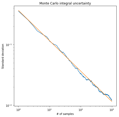
This is telling us that the variance of our estimator scales as $1/\sqrt{N}$. The image below shows the standard deviation of a 1000 estimates of the integral for different numbers of points used when evaluating it. As expected, the standard deviation of our estimates goes down as $1/\sqrt{N}$.

Note that despite me calling it an error all the time is not a bound on the eror we are making. When we make a MC estimate of an integral we are sampling a realization of a random process. The variance of said process is what we are calculating. If the variance is small the estimates from consecutive MC estimates will likely be close to each other.

Assuming our integration domain is the unit cube which we can always do because it is just a simple variable change away from us.

$$\sigma^2(f)=\int \mathrm{d}x \; [f(x)-I]^2$$

$$\sigma^2(f)=-2I^2 + \int \mathrm{d}x \; [f(x)^2 + I^2]$$

$$\sigma^2(f)=\int \mathrm{d}x \; f(x)^2 - I^2$$

On the other hand

$$ \int \mathrm{d}x_1 \dotsb \int \mathrm{d}x_N \left(\frac{1}{N} \sum f(x_i) - I\right)^2$$

Expanding the square we get

$$ I^2 -2I \int \mathrm{d}x_1 \dotsb \int \mathrm{d}x_N \frac{1}{N} \sum f(x_i) +\int \mathrm{d}x_1 \dotsb \int \mathrm{d}x_N \left(\frac{1}{N} \sum f(x_i)\right)^2 $$

For the first of those integrals we can change the order of the sum and the integration to get:

$$\frac{1}{N} \sum \int \mathrm{d}x_1 \dotsb \int \mathrm{d}x_N \; f(x_i)$$

All those integrals evaluate to $I$ for one of them and the rest evaluate to 1 so the sum of integrals is just $IN$ and we are left with:

$$ -I^2 + \int \mathrm{d}x_1 \dotsb \int \mathrm{d}x_N \; \left(\frac{1}{N} \sum f(x_i)\right)^2 $$

For the last integral we have to once again expand the square of the sum. We will be left two terms, one corresponding to the square of each element and another one with products of the form $f(x_i) f(x_j)$

$$ \frac{1}{N^2} \int \mathrm{d}x_1 \dotsb \int \mathrm{d}x_N \; \left(\sum f(x_i)\right)^2 $$

$$ \frac{1}{N^2} \int \mathrm{d}x_1 \dotsb \int \mathrm{d}x_N \; \left(\sum f(x_i)^2 + 2 \sum f(x_i)f(x_j)\right) $$

Were the factor 2 comes by because each mixed product appears twice in the sum. Now we are free to break everything into 2 integrals of sums and we can reverse them as we did before. The first of them will be:

$$\frac{1}{N^2}N \int \mathrm{d}x \; f(x)^2$$

The terms of each sum will integrate to $I^2$ and ther are $\frac{N(N-1)}{2}$ of them and hence that second integral is:

$$2 I^2\frac{1}{N^2} \frac{N(N-1)}{2} $$

Putting it all back together we find that the equation we started from is equal to

$$\frac{\sigma^2(f)}{N}$$

We can even make use of an estimate of the function variance in order to make an algorithm that will automatically select the number of points that need to be used.

This is demonstrated in the code below. We first generate estimates for the integral and the variance using our Monte Carlo estimates and based on that compute how many additional function evaluations we should do in order to go under some error. The process is repeated until we hit an error estimate that is below our settings.

Stratified Sampling

Reached this point most would be satisfied, but if you've been following closely enough, you may have noticed that when doing the Monte Carlo integral we have been a bit wasteful. In the example with the step function above most of the function evaluations gave us very little information about the integrand, they either evaluated to 2 or 0. All the interesting things happen around the jump. This is idea is intuitively captured by the equation that describes the variance of the estimator. On the flat regions of the function the variance is very small (0) so if we focused only on those regions the estimate for our error estimates would be equally small after a small number of evaluation. However, in regions of high variance, e.g. close to the discontinuity, we need more evaluation in order to reach the same error.

That last observation inspires a strategy to reduce variance by sampling more frequently regions of greater variance. The basic idea is to divide the integration region into subregions and add the partial results from each one of them. We do so while doing more function evaluations in those subregions where we think that the function changes more in order to smooth out the error and use our finite computational resources more efficiently.

Assuming we break our integration region $M=[0,1]^D$ into $k$ regions $M_j$ where $j=1,\dotsb ,k$ and that we perform integration on region with $N_j$ points our estimate for the integral is:

$$E = \sum^k_{j=1} \frac{\mathrm{vol}(M_j)}{N_j}\sum^{N_j}_{n=1}f(x_{jn})$$

To proof that this is the case we start by observing that

$$\int_M \mathrm{d}x \; f(x) = \sum_j \int_{M_j}\mathrm{d}x \; f(x)$$

which follows trivially from the definition of the Riemann integral. Now suppose that the constant integration boundaries along each dimension for region $M_j$ are the following set of pairs which represent the lower and upper boundaries for it along each dimension

$$\{(a_{jd},b_{jd})\}_{d=1}^D$$

We now have to solve integrals of the form:

$$ \int_{a_{j1}}^{b_{j1}} \mathrm{d}x_{1j} \dotsb \int_{a_{jN}}^{b_{jN}} \mathrm{d}x_{Nj} \; f(x_j)$$

We can introduce the variable transformation

$$y_j = \frac{(x_j-a_{jd})}{(b_{jd}-a_{jd})}$$

This brings back all the integration limits to the unit hypercube but they are now scaled by a factor equal to the original volume of the $M_j$ space.

$$ \mathrm{Vol}(M_j) \int_0^1 \mathrm{d}y_{1j} \dotsb \int_0^1 \mathrm{d}y_{Nj} \; f(y_j(b_{jd}-a_{jd})+a_{jd})$$

with

$$\mathrm{Vol}(M_j) = \left(\prod_d (b_{jd}-a_{jd}) \right)$$

Here I'm a bit loose with the notation for the argument to $f$ note that there are $D$ arguments in total all transformed in a similar way. Almost there. Lets rename $y$ to $x$

$$\sum_j \int_{M_j}\mathrm{d}x \; f(x) = \sum_j\mathrm{Vol}(M_j) \int \mathrm{d}x \; f(x(b_{j}-a_{j})+a_{j})$$

Doing now the Monte Carlo estimate for each integral

$$ \sum_j \frac{\mathrm{vol}(M_j)}{N_j}\sum^{N_j}_{n=1}f(x_{jn}(x(b_{j}-a_{j})+a_{j}))$$

With $x_j\sim U(0,1)$ so if we work under the assumption that we are taking the points from our original subpaces we can more cleanly write the result as

$$ \sum_j \frac{\mathrm{vol}(M_j)}{N_j}\sum^{N_j}_{n=1}f(x_{jn})$$

which is what we were after. The proof also makes explicit how we have to transform our samples from the random number generator before feeding them into the function for performing the Monte Carlo integration.

A proof almost identical to the one above allows us to show that the variance of the subdivided integral is:

$$ \sum_j \frac{\mathrm{vol}(M_j)^2}{N_j}\sigma^2 (f) |_{M_j}$$

So we intuitively know that by breaking the integral into subregions and sampling more frequently regions of higher variance we will get a better integral estimtate for the same number of function evaluations. But how to choose the points we want to allocate to each region?

We can gain some intution by considering the following 1D integral which we have subdivided into to regions $M_0=[0,1/2]$ and $M_1=[1/2,1]$. Accordingly the estimate of the variance for the whole integral is:

$$\frac{1}{4}\left(\frac{\sigma^2(f)|_a}{N_a} + \frac{\sigma^2(f)|_b}{N_b}\right )$$

which is minimized for fixed $N=N_a + N_b$ by choosing

$$\frac{N_a}{N} = \frac{\sigma (f)|a}{\sigma (f)|a+\sigma (f)|b}$$

By being smart with respect to what region we sample more often we can reduce the variance of the whole integral and therefore require less evaluations to reach the same error.

MISER algorithm

We would like to have now an adaptive algorithm that made use of stratified sampling. The first thing that came to my mind was the following algorithm.

Split the integration region along each dimension and do a Monte Carlo integral with N points on each of them.
For each region, if the estimate error of a region is smaller than our target error we stop. Otherwise, we recursively go to 1.

Despite any number of minor improvements this algorithm has one fatal flaw. The curse of dimensionality rears its head in step 1. Each subdivision step creates $2^D$ subregions which will become impossible to track very quickly. We need to do better.

One possible fix for this problem is to only split along one dimension; the one that would brings that biggest reduction in error. This is precisely what the MISER algorithm trys to accomplish.

Here I show a slightly simplified version of the one presented in the FORTRAN code of the original article. It more closely resembles the algorithm as described by the equations and main text of the original. The original FORTRAN implementation introduces a modified and more robust estimator for the variance in each region, as well as a dithering parameter that is used to break the symmetry of the partitions. This improves the performance when the integrand has symmetries that match those of the split regions.

MISER is a recursive algorithm that consists of two main phases. During the first one we explore the integrand looking for areas of high variance. We call this the variance exploration phase. During the second phase the algorithm evaluates the value of the integral of each of the subregions generated depending on the variance we estimated during phase 1.

The algorithm has four main parameters that control it's behaviour: N_points, MNBS, MNPTS, pfac and alpha.

The first of them N_points fixes our function evaluation budget. By the end of the algorithm we will have sampled the integrand N_points times.

MNBS fixes the cutoff point at which we decide to switch from phase 1 of the algorithm (variance exploration) to phase 2 (actually computing the integral).

With MNPTS we decide what is the minimum number of points that are going to be used during a phase 1 step. If it is set to low, the estimates we generate for the variance of each region will be worst and domain in the integral won't be split well into subregions. On the other hand, if we set it to high we will do great at exploring the variance landscape of the integral but by the time we reach phase 2 we won't have evaluation budget to do a good estimate of the integral. As usual the optimal place lies somewhere in the middle and it requires a bit hand tuning although sane defaults are available.

pfac specifies what fraction of the points remaining are used during the variance exploration phase. Similar caveats as to how to set up MNPTS apply here. The original publication recommends to use a value of 0.1 and the libraries I've found around stay true to it.

Finally, with alpha controls how many points end up on each of the splits. The basic formula for the optimal split doesn't strictly apply any more due to the recursive nature of the algorithm. So we adjust via alpha which is empirically chosen.

With the parameter description out of the way let's dive into the actual implementation and check how MISER works in detail. The function below describes the core of the algorithm.

The variance exploration phase is taken care of in the else branch and it's always the starting point. It can be summarized as follows:

Compute how many points to use for this variance exploration step. As we saw above this will depend both on pfac and MNPTS. (line 23)
Decide along which dimension we are going to split in halve the domain. (line 26)
Allocate how many points of our remaning evaluation budget we are going to use to explore each of the halves of the domain. (lines 29 to 32)
Recurse into each of the halves by running the algorithm again on each of the halves with the correct evaluation budget associated to each of them. (lines 35 and 36)
The recursion is broken when the budget goes below MNBS. In that case we combine our integral estimates for each halve and go up the recursion stack recursively doing so. (lines 30 and 40).

This bullet points can be directly translated into code as follows:

With the core ideas of the algorithm defined let's look know at each of the individual components.

The variance exploration is completed when the remaining function evaluation budget is below MNPTS. If this is the case we simply run a vanilla Monte Carlo like the one we defined befor which will over the subregion we are working on. This is taken care of by the mc_kernel function. It returns both the integral and variance estimates of the integral over a region of the domain. This serves two purposes. Firstly, it will provides us with an estimate of the error we are making. Also, it makes the recursion easier to work with because both branches have the same return values.

Now, if instead we have enough function evaluations remaining in our budget we have to decide along which dimension we will split the subregion of the domain that we are exploring. The _split_domain method is responsible for this.

This one takes another parameter alpha.

Finally, we can put it all together into a single class that demonstrates the method. As usual, the full code can be found at GitHub.

Trying to integrate a donut shaped function clearly shows that at the edges of the function, where it changes faster and therefore the variance is higher the function is sampled much more often than on the flat regions.

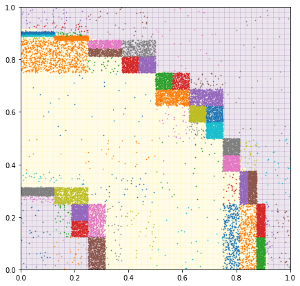
Points used by MISER for the integral evaluation.

This completes our whirlwind tour of Monte Carlo methods as they apply to integration. If you've enjoyed it just ping me :)

Outro

If you ever need to use plain Monte Carlo or MISER you will be better of trying scikit-monaco, written in Cython, or the always trusty GSL. This libraries provide robust and fast implementations of the algorithms described above and more. For instance, GSL also provides the VEGAS algorithms which can improve the accuracy of the integral estimate when the integrand can be approximated by a product of 1D functions.

$$\vec{f}(\vec{x})=\prod_{i=1}^D f_i(x_i)$$