Maxwell Rules - Homographies: Looking through a pinhole

Homographies: Looking through a pinhole

Ever wondered how you can match the pixel coordinates on an image to actual coordinates on the world? This post is for you! By the end of it you will know how to construct (and derive) a relationship between the two. Most remarkably it all boils down to multiplying a bunch of 4x4 matrices.

To get started we first need to build a model of how our camera works. In other words, we need to be able to find where on the sensor a ray of incoming light will hit it.

The camera model

Lets start by assuming that we have a perfect aberration free optical system. Despite the long list of adjectives this is a pretty good approximation for many optical systems. Having accepted this, any optical system can be characterized by its cardinal points. For our purposes we are interested on the rear and frontal nodal points and the back focal plane. Quoting wikipedia the nodal points are those that have the property that a ray aimed at one of them will be refracted by the lens such that it appears to have come from the other, and with the same angle with respect to the optical axis. The image below shows the nodal points for two optical systems: a thick lens and a more complicated camera.

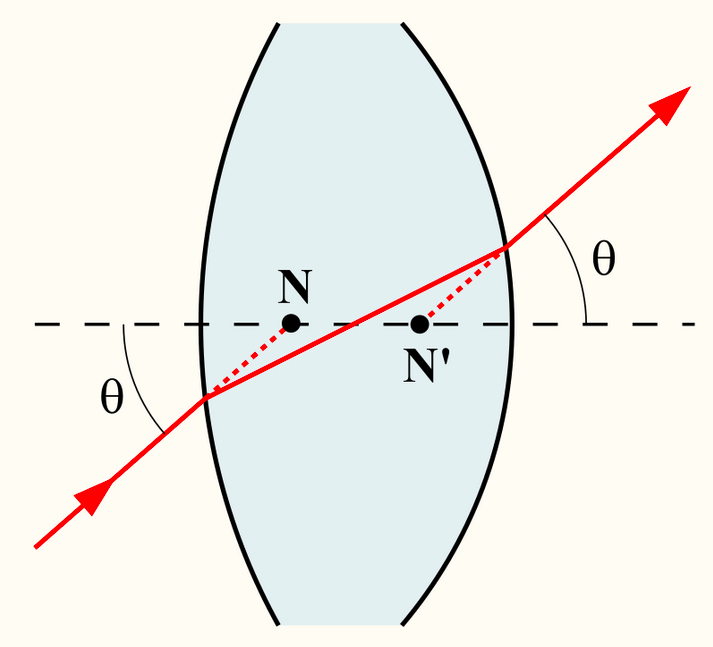Thick lens [1].

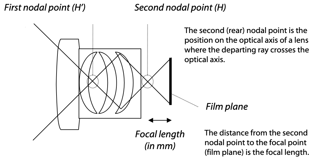Complex camera system [2].

Next we need to consider the back focal plane. All the light coming from a distant point in the scene will converge somewhere on the focal plane. This is where the image is formed and where we have to place the camera sensor. We will call the focal distance, $f$, to the distance between the rear nodal point (the one closest to the sensor) and the back focal plane.

Since all the light rays coming in at a fixed angle into the system are focused on the same point of the focal plane and all the ray hitting the front nodal point "comes out" at the same angle from the rear nodal point it shouldn't take much convincing to accept that we can model where rays coming from the scene are going to hit the sensor as in the image below.

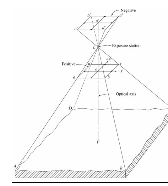Pinhole camera model

In order to find the actual place on the sensor a distant point will be imaged to we just need to draw a line from the point on the scene to the rear nodal point of the optical system. The point of intersection between the positive in the image above and line corresponds to where the scene point will be focused on the camera sensor. It all boils down to intersecting lines and planes.

Camera position and sensor coordinates

The positive, from now onwards the sensor plane, is located at a distance $f$ (the focal length) from the frontal nodal point. Given a normalized vector describing the normal of the sensor plane $\vec{n_s}$ and the position of the frontal nodal point $\vec{c}$ we can fully describe the camera. The vector $\vec{n_s}$ represents both the pointing direction of the camera and the normal of the sensor plane. To fully describe the position of the sensor plane we also require a point in it. One such point is obtained by moving away from the frontal nodal point by a distance equal to the focal length, that is:

$$\vec{c} + f\vec{n_s}$$

Next to characterize any point within the sensor plane we need to select two directions perpendicular to $\vec{n_s}$, let's call them $\vec{s_x}$ and $\vec{s_y}$. Since these two vectors will also represent the coordinate basis for the sensor the most logical choice is to select vectors parallel to the rows and columns of the sensor. In this way any point on the sensor plane can be represented by two numbers $(S_x, S_y)$ as follows:

$$\vec{s} = \vec{c} + S_x \vec{s_x} + S_y \vec{s_y} +f \vec{n_s}$$

Note that above we have given double duty to the point $\vec{c}$; it's both acting as an ordinary point on the sensor plane to fully characterize it and as the origin of the coordinate system we are defining for it.

Finally, for maximum convenience we could (but won't here) rescale the length of $\vec{s_x}$ and $\vec{s_y}$ so that it matches the width and height of the sensor respectively. With this choice the vertical edges of the sensor are placed at $S_x=\pm 0.5$ and the horizontal ones at $S_y=\pm 0.5$. Another very practical alternative is to make the length of the in plane vectors for the sensor equal to the pixel size, like this we would be able to express $(S_x, S_y)$ in units of pixels.

The world plane

The homographies we are interested on relate points belonging to two planes. On one hand we had the sensor plane and on the other hand we have what I call here the world plane. As with the sensor plane, the world plane can be described by a point in it, $\vec{w_o}$ and it's normal, $\vec{n_w}$. And again, as with the sensor plane we can repurpose the selected point on the plane as the origin for it's intrinsic coordinate sytem. With this in mind any point on the world plane can be described by two numbers $(W_x, W_y)$

$$\vec{w} = \vec{w_o} + W_x \vec{w_x} + W_y \vec{w_y}$$

$\vec{w_x}$ and $\vec{w_y}$ can be any two vectors as long as they are not colinear and they are perpendicular to $\vec{n_w}$, however, often there is a natural choice for them. In my domain, GIS, the world plane x and y would be usually pointing north and east.

Sensor ⟺ World mapping

We are going to be dealing with lines and planes intersecting each other so dusting out the line-plane intersection equation sound like a sensible thing to do:

$$\vec{w_i} = \vec{c} + \frac{(\vec{w_o}-\vec{c})\cdot\vec{n_w}}{\vec{r}\cdot\vec{n_w}}\vec{r}$$

In the equation above $\vec{c}$ reprents a point along the line, next $\vec{r}$ is the vector defining the direction of the line, $\vec{w_o}$ is a point on the plane we are intersecting and $\vec{n_w}$ is the normal to the plane. Note that we have reused symbols from the previous sections.

According to our camera model, to find the point on the world plane corresponding to a point on the sensor we need to draw a ray starting on the camera frontal nodal point ($\vec{c}$) and passing through a point on the sensor ($\vec{s}$). Using the coordinate system we used above for the sensor the direction vector for any such ray can be describe as:

$$\vec{r} = \vec{s} - \vec{c} = S_x \vec{s_x} + S_y \vec{s_y} +f \vec{n_s}$$

Using the ray-plane intersection equation above we now have the world position for any point on the sensor. Next we want to figure out how that point is expressed on the coordinate frame attached to the world plane. For this, first shift the intersections so that they are referenced to the origin of the world plane which leaves us at:

$$\vec{w_i}-\vec{w_o} =\vec{c} - \vec{w_o} - \frac{(\vec{w_o}-\vec{c})\cdot\vec{n_w}}{\vec{r}\cdot\vec{n_w}}\vec{r}$$

or after defining $\vec{\delta} = \vec{w_o} - \vec{c}$:

\begin{equation} \vec{w_o}-\vec{w_i} =-\vec{\delta} + \frac{\vec{\delta}\cdot\vec{n_w}}{\vec{r}\cdot\vec{n_w}}\vec{r} \end{equation}

The final touch is to project $\vec{w_o}-\vec{w_i}$ on the $x$ and $y$ coordinates of the world reference frame. This is simply done taking the dot product of $\vec{w_o}-\vec{w_i}$ with $\vec{w_x}$ and $\vec{w_y}$.

Time for some code! First some preliminaries and definitions. We will need some structs to represent the planes and the camera. A plane is characterized by a basis and a point it passes through. The first two vectors of the basis must be perpendicular to the third which is the normal to the plane. For a camera the point defining its sensor plane is implicitly defined by the focal length and the camera position.

We also have a little helper function to rotate the camera with an XYZ rotation and then define a camera with at a more or less arbitrary position and the world plane.

Implementing the line intersection is straightforward. We will not spend any time optimizing or refactoring any of this because there is a much better alternative. The code below makes use of the observations that the ray vector can conveniently expressed by arranging the basis of the sensor plane as the columns of a matrix which we will call $B_s$:

$$ \vec{r} = \left( \begin{array}{cccc} | & | & | \\ \vec{s}_{x} & \vec{s}_{y} & \vec{n}_{s} \\ | & | & | \end{array} \right) \left( \begin{array}{c} S_x \\ S_y \\ f \end{array} \right) = B_s \left( \begin{array}{c} S_x \\ S_y \\ f \end{array} \right) $$

On a first glance this looks like the end of the road. The equation above can't be simplified any further and can't certainly be expressed as a linear operation (i.e. just a matrix multiplication) because we have some stuff dividing that depends on the input and also some vector additions. But this is a post about homographies and I haven't even named them yet so lets see what we can do.

Homogenous coordinates

Before speaking about homographies we should introduce homogenous coordinates, this were invented by Möbius (same one as the infinite strip). Through a clever trick they allow us to express affine transformation, i.e.:

$$ y = Ax + b $$

using a single matrix multiplication. This black magic is accomplished by expanding the matrix with an additional dimension. In the 3 dimensional case it works out like this, but generalizing to other dimensions is trivial.

$$ \begin{pmatrix} &\LARGE A & & \begin{matrix} b_1 \\ b_2 \\ b_3 \end{matrix}\\ 0 & 0 & 0 & 1 \end{pmatrix} \left ( \begin{array}{c} x_1 \\ x_2 \\ x_3 \\ 1\end{array}\right) $$

You can try it and check that it does indeed represent the transformation above, the bottom element of the output is always 1 and can be discarded. The reason for this is that we have $(0\;,0\;,0\;,1)$ on the bottom row, but what if it were something more general, say,$(h_x\;,h_y\;,h_z\;,h_t)$? In that case, the bottom element of the output vector would not be one. To go back to normal coordinates then all you would have to do is renormalize your vector so that the last element is one, and then discard the one to go back to 3D.

$$ \begin{pmatrix} x'\\ y'\\ z'\\ t' \end{pmatrix} \rightarrow \begin{pmatrix} x'/t'\\ y'/t'\\ z'/t'\\ 1 \end{pmatrix} $$

The extra free parameters make it possible to express more general transformations. The new bigger family of transformations enabled are called homographies. The most important thing to note is once all is said and done we end up with a non-linear transformation because each of the components of the vector can now be divided by a linear combinations of the components of the input vector.

Reexpressing everything

Wait you said divide by a linear function of the inputs? Yes I did! Hmmm, let me have a look again at the line-plane intersection equation. Certainly, here it is:

\begin{equation} \frac{\vec{\delta}\cdot\vec{n_w}}{\vec{r}\cdot\vec{n_w}}\vec{r} \end{equation}

So the numerator is just a constant number that depends on the problem setting. Just a constant scaling. That's easy to express as a matrix, in non-homogenous coordinates it is just the identity matrix multipled by a scalar. Next we have $\vec{r}$, which we already figured out how to express as matrix multiplication in the Sensor ⟺ World mapping section. Finally, let's have a look at the denominator:

$$ \vec{r}\cdot\vec{n_w}=(S_x \vec{s_x} + S_y \vec{s_y} +f \vec{n_s})\cdot\vec{n_w} $$

now we plug in the equation for $\vec{r}$ that we worked out on the Sensor ⟺ World mapping section. We have:

$$ (S_x \vec{s_x} + S_y \vec{s_y} +f \vec{n_s})\cdot\vec{n_w}= (\vec{s_x}\cdot\vec{n_w},\; \vec{s_y}\cdot\vec{n_w},\; 0,\; f \vec{n_s}\cdot\vec{n_w})\left( \begin{array}{c} S_x \\ S_y \\ 0 \\ 1 \end{array} \right) $$

On the second equality I have added an extra element to our vector that corresponds to an $S_z$ coordinate that we will ignore but makes the matrix algebra work, bear with me.

Lets write what we have so far as matrix using homogenous coordinates:

$$ \begin{pmatrix} &(\vec{\delta}\cdot\vec{n_w}) \LARGE B_s & & \begin{matrix} 0 \\ 0 \\ 0 \end{matrix}\\ \vec{s_x}\cdot\vec{n_w}& \vec{s_y}\cdot\vec{n_w}& 0& f\vec{n_s}\cdot\vec{n_w} \end{pmatrix} \left ( \begin{array}{c} S_x \\ S_y \\ 0 \\ 1\end{array}\right) = H_0 \left ( \begin{array}{c} S_x \\ S_y \\ 0 \\ 1\end{array}\right) $$

The bottom row will produce the denominator that once we "normalize" the output will produce exactly the formula we want to replicate. Nice!

Now we need a shift by a $-\vec{\delta}$, as we saw before this can be expressed with an identity matrix where we adjust the last column to perform the shift:

$$ H_1 = \begin{pmatrix} 1 & 0 & 0 & -\delta_x \\ 0 & 1 & 0 & -\delta_y \\ 0 & 0 & 1 & -\delta_z \\ 0 & 0 & 0 & 1 \end{pmatrix} $$

As before we still need to reproject on to the world coordinates basis. In essence this consists on taking the dot product of the results from $H_1 H_0$ with the 3 basis vectors of the world coordinate system. Arranging the world coordinate basis vectors as rows accomplishes exactly this.

$$ B_w = \left( \begin{array}{cccc} | & | & | \\ \vec{w}_{x} & \vec{w}_{y} & \vec{n}_{w} \\ | & | & | \end{array} \right) $$

And setting this up on homogenous coordinates produces:

$$ H_2 = \begin{pmatrix} &\LARGE B_w^T & & \begin{matrix} 0 \\ 0 \\ 0 \end{matrix}\\ 0 & 0 & 0 & 1 \end{pmatrix} $$

All of this can be translated into code as follows:

And that's pretty much it. The generated matrix will translate points on the sensor to coordinates on the world plane. One of the big improvements of doing things this way is that the inverse transformation that takes us from ground to sensor is now trivial, all we have to do is find the inverse of the previous homography.

And that is basically it for the math and the code.

Going further

On a real applications you want to make some further considerations.

More vectorization: The code above acts on single points. We can act on more of them simultaneously by arranging our points of interest into a matrix. Difficulty: EASY
We are refering all the time to a coordinate system on the sensor (Sx, Sy) which is centered on it and that has length units as it maps spatial positions over the physical sensor. This is a bit awkward, at the very least we want to work with some normalized coordinates over the sensor. One way to do it is to scale the sensor coordinates in such a way that the sensor corners are mapped to the points $(\pm 0.5, \pm 0.5)$. For this we just need to scale $S_x$ and $S_y$ with the physical length of the sensor. This just a matrix multiplication away.

$$ H_s = \begin{pmatrix} 1/L_x & 0 & 0 & 0 \\ 0 & 1/L_y & 0 & 0 \\ 0 & 0 & 1 & 0 \\ 0 & 0 & 0 & 1 \end{pmatrix} $$

And

$$ H_2 H_1 H_0 -> H_2 H_1 H_0 H_s $$