Image transformations: Peeking under the hood

Raw aerial imagery (or any kind of imagery) always suffers from perspective distortion. You've probably noticed how those helicopter shots over Manhattan have that distinctive look where the buildings seem to lean away from the camera. In the realm of GIS, this perspective can make it incredibly challenging to measure distances and angles on the image accurately. Moreover, comparing images taken from different positions and camera orientations becomes a puzzle. In order to work around this, images need to be transformed in such a way that they are made consistent with each other.

Below I will describe the process of how given a coordinate transformation one can take an image and transform it. For the purpose of this post we will assume that we have been given such a transformation and will focus on the mechanics of how to transform the image.

What is a coordinate transformation?

Today an image transformation will be be a function \(f(x,y): \mathbb{R}^2 \rightarrow \mathbb{R}^2\). That is, a function that maps some coordinates \((x,y)\) to some other point \((x',y')\).

Theory

Now, let's create an image (I could have used some pre-made image, but where's the fun in that?) and define the transformation we want to apply to it.

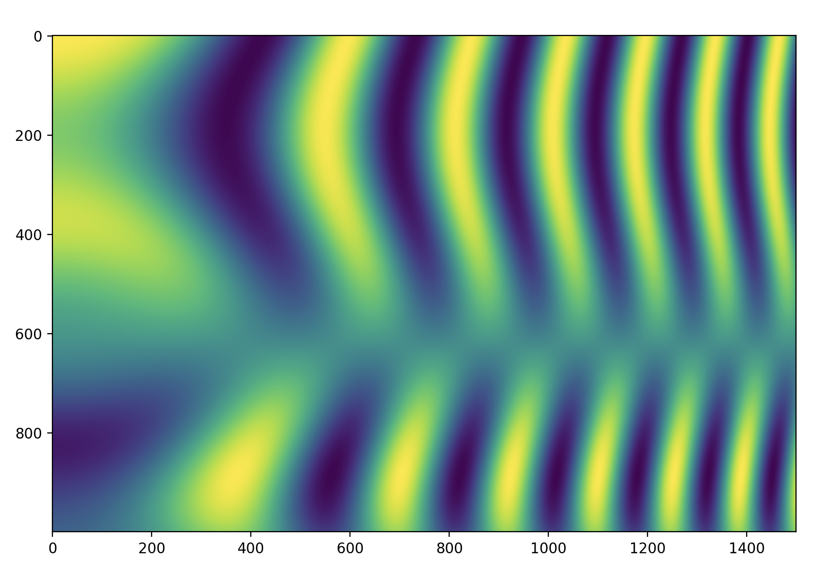
So that's our input image.

Lets now think about the transformed image as an empty canvas whose pixels we need to colour in. Once finished this canvas should show the transformed input image after having applied the transformation \(f\). Now, consider the pixel \((i', j')\) from the transformed image. What colour do I pick? This wasn't obvious to me at first until I realized that it could be rephrased as: What pixel from the source image did pixel \((i', j')\) came from? This is easier because we have a transformation that maps pixel coordinates on the source image to pixel coordinates on the transformed image. That is, if:

then

.

As we will discuss later, being able to invert the transformation quickly is really important in order to be able to implement image transformations efficiently.

The rest is easy. All that needs to be done is to iterate over all the pixel coordinates of the transformed image, put them through \(f^{-1}(i',j')\) and query the source image at the position we got to figure out the value of each pixel. Not all the coordinates that we put through \(f^{-1}\) will end up just on top of of a pixel on the source image with nice and round integer coordinates. In fact almost none will. To get around it we will make use of interpolation. Here, is where insisting on using \(f^{-1}\) as opposed to \(f\) really pays its dividends. Notice that the image we are querying is (in a certain world view) just data arranged into a neat rectangular and very regular grid. It is this fact what allows all kinds of interpolation algorithm to be built very efficiently.

Enough speaking show me the code!

Code

The goal of the listing below is to identify the bounds of the transformed image. To this end, it calculates all the pixel coordinates around the edges of the image (lines 30:33), puts them through the (forward) transform (lines 36:41) and finally computes the mins and maxs (lines 44:45).

Next task up is to build the coordinates of the transformed image (lines 1:10). The arrays have been flattened so that apply_affine gets an array of size \((2, N)\) with N being the number of pixels. Then, apply the inverse transform to those coordinates to figure out what pixel in the source image they came from.

Finally, build an interpolator over the original image (lines 18:23), notice that we are using np.arange(rows) and np.arange(cols), and sample it at the transformed positions, target_coords_at_source (line 24).

Here is the result a transformed image.

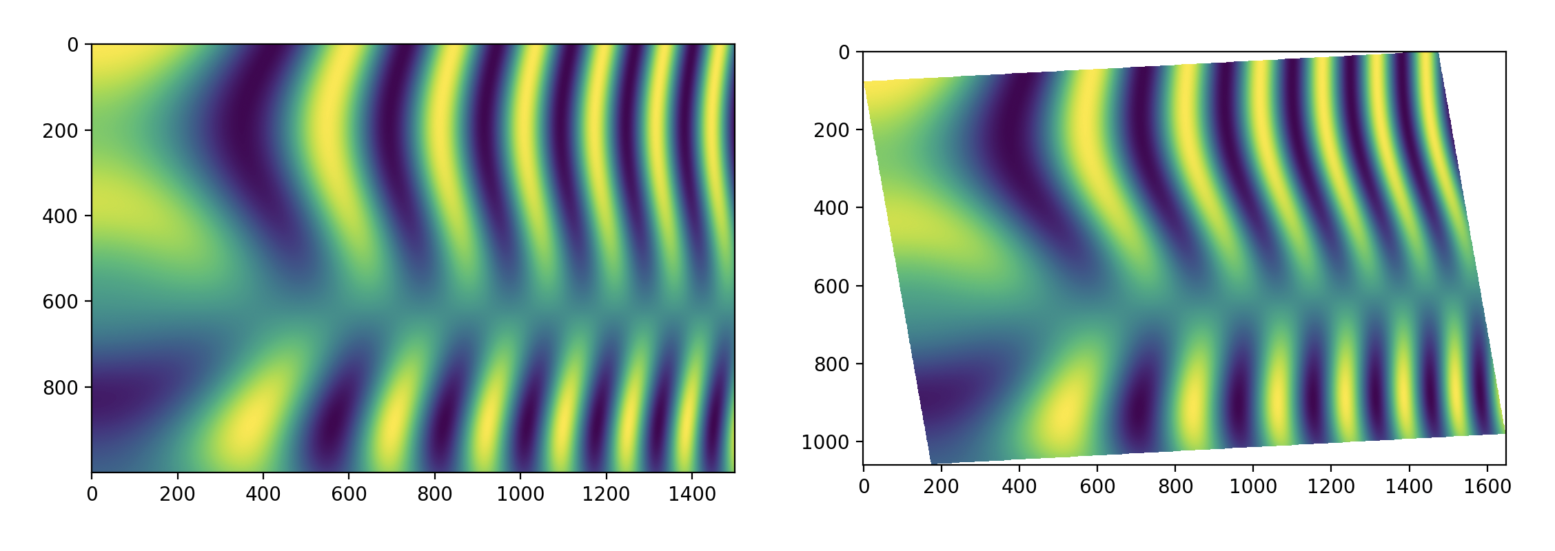
Happy transforming! ...... hey hey wait. I insist on using the forward transform. Okay, here we go.

Using the forward transform

Up there I really made my life much easier using an affine transformation as it meant I could very easily invert it. However, this won't be the case for many coordinate transformations you will find out in the wild. Either the relevant equations are too complicated, there are straight up no equations or the function is just not invertible. So what to do if you don't have that luxury? This is the case for even simple transformations like second order polynomials. In some cases they may be invertible if constrained to a finite domain but you still wont get a closed form equation for the inverse.

Here are some options!

Bring your own inverse

Often times, it is yourself who is calculating the transformation based on some points that have been extracted from two images. The laziest solution is two invert the roles of the two set of points so that what used to be image 1 is now image 2 and viceversa. This will cheaply get you your inverse.

Iteratively find the inverse at each pixel coordinate

A more costly, but usually much more accurate way to go about it, is to use a root finding algorithm (e.g. Newton's method) to find \((i, j)\) such that:

for every \((i',j')\). This may sound ridiculously expensive but is not, particularly when compared to the next option we will show. One of the reasons for it not being too bad is that, assuming your transformation is nice, you can use the solution from a neighbouring pixel to seed the iterations for your current position greatly enhancing convergence.

Create some sort of approximation to the inverse

This option requires the most cleverness, in exchange you get (often) error bounds and closed form formulas. The one case I know for this is are the simplified 😂 equations for the UTM transformations, go check them out.

The forward transform or nothing

One way of thinking about the forward transform is as follows: Where should I move the RGB at pixel position \((i,j)\) too? Under this point of view, our transformation creates a new non-regular grid of data. We can then interpolate over this new grid at the integer coordinates of the output image to generate it.

That's it! Nice and intuitive! Well not so fast... not so fast indeed. Since this grid is non-regular, that is, not placed in a rectangular arrangement we now need to fetch an interpolation algorithm capable of dealing with this situation. One such example is LinearNDInterpolator. That works but there is an awful lot of work happening under the hood, for starters it is building a Delaunay triangulation of your data and just that is going to take a long time when we start talking about 1 megapixel images.

Outro

That's a wrap for today! Hopefully, you found this journey through image transformations as helpful as I did. And remember, when possible, try your best to avoid the forward transform!